【NIPS2019】Infidelity and Sensitivity：模型可解释性方法的定量评估

如何模型可解释性方法的评估？

模型可解释性方法的评估可以分为主观度量和客观度量两种，可解释性本身是偏人本身的一个概念，因此目前占主流的评估方法为主观度量，但是完全依靠人的主观度量评估模型可解释性方法是不可行的。文章便提出了依靠客观度量去评估模型可解释性方法的两个重要度量 Infidelity 与 Sensitivity 。

Infidelity--失真度

1. 完整性公理

Infidelity的定义来源于Ancona ^[1] 中的completeness axiom(完整性公理)，定义如下：

设模型对应函数 f(x) ，输出feature importance的可解释性方法函数 \Phi(f,x) ， I 定义为对输入 x 的扰动，则完整性公理的公式如下：

I^T\Phi(f,x)=f(x)-f(x-I)

因此完整性公理视最佳可解释性方法函数 \Phi(f,x) 为扰动 I 下模型输出 f(x) 对输入 x 的导数。

2 . Infidelity的定量表示

设扰动 I\in\ R^d 为一随机变量，对应的概率分布为 \mu_I ,Infidelity的定量公式表述为：

INFD(\Phi,f,x)=E_{I\in \mu_{I}}[(I^T\Phi(f,x)-(f(x)-f(x-I)))^2]

假定满足完整性公理的可解释性方法函数 \Phi^*(f,x) ， Infidelity衡量便是可解释性方法函数 \Phi(f,x) 与 \Phi^*(f,x) 之间距离期望，该距离期望越小，失真度infidelity越小 。

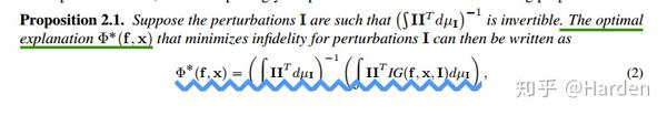
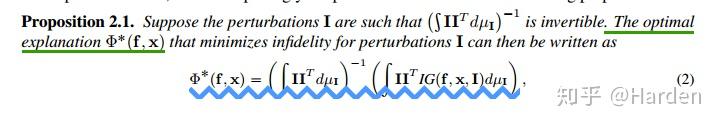
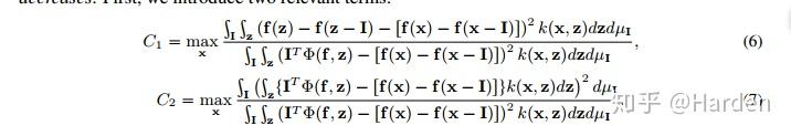
3. Explanations with least Infidelity

Infidelity度量下，最佳的可解释性方法函数 \Phi^*(f,x) 定义如下，

Integrated Gradient ^[2] 的公式为 IG(f,x,I)=\int_{t=0}^{1}\nabla f(x+(t-1)I)dt ,

Smoot Gradient ^[3] 的泛化公式为 \Phi_{k}(f,x)=[\int_{z}k(x,z)]^{-1}\int_{z}\Phi(x,z)k(x,z)dz ， 其中 k(x,z) 为高斯核函数，同时还可以是其他形式的核函数。

因此可以看出，具有least infidelity的可解释性函数 \Phi^*(f,x) 是Integrated Gradient的平滑版本，对应的核函数形式为 II^{T}

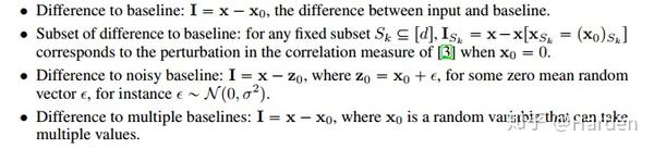
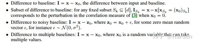
扰动 I 有多种定义形式，如下四种扰动：Difference to baseline, Subset of difference to baseline, Difference to noisy baseline, Difference to multiple baselines

3. Many Recent Explanations Optimize Infidelity

有许多模型可解释性方法可以认为是对给定的扰动 I 约束下，优化infidelity度量。

(1)固定基线扰动: I=x-x_0 ,此时扰动固定，对应的可解释性方法有Integrated Gradient, Deep Lift ^[4] , LRP ^[5]

(2)固定坐标扰动： I=\epsilon\cdot e_i ， e_i 是一个坐标向量偏置

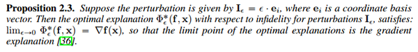
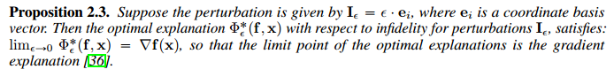
此时的最佳可解释性函数可以认为是梯度可解释性函数 ^[6]

： lim_{\varepsilon\rightarrow0}\Phi_{\varepsilon}^{*}=\nabla f(x)

(3)非固定坐标扰动： I= e_i\odot x ， e_i 是一个坐标向量偏置

此时最佳的可解释性函数可以认为是occlusion-1 explanation ^[7]

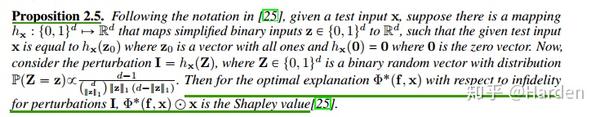
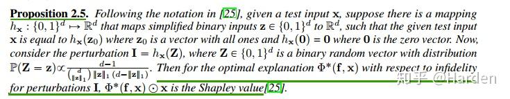
(4)0-1 mask扰动：设模型输入 x\in\{0,1\}^d ，此时扰动定义为 I=h_x(z), z\in\{0,1\}^d

此时最佳解释函数 \Phi^*(f,x) 与输入 x 的逐点乘积等于Shapley value ^[8]

4. Some Novel Explanations with New Perturbations

论文作者提出了一些新的扰动形式，基于该些扰动的可解释性方法在Infidelity和Sensitivity两个维度上都取得最佳效果

(1)noisy baseline: 是对固定基线扰动 I=x-x_0 的一种改进，此时 x_0 变为一个随机变量 z ，例如高斯噪声。

(2)Square remove：针对图像的扰动，对图像中的一部分或者数个部分的像素块进行mask。

5. Local and Global Explanations

Local Explanation关注的是模型输出对输入feature变化的敏感度

Global Explanation关注的是输入feature变化导致的模型输出的变化。

Sensitivity-敏感度

论文将Sensitivity定义为可解释性方法函数 \Phi(x) 对输入 x 的导数，具体的表达如下：

首先定义 [\nabla_x \Phi(f,x)]_j ，其中 j\in \{1, 2 ... d\}

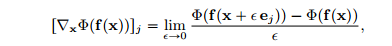
可得基于梯度的敏感性分数 SENS_{grad}(f,x,\Phi,r) 的公式表达为：

由此得到基于Lips系数的敏感性分数表达 SENS_{lips}(\Phi,f,x,r)

如果可解释性函数的局部满足Lipshitz continuous，我们可以得到最终的敏感性分数 SENS_{MAX}(\Phi,f,x,r) 表示

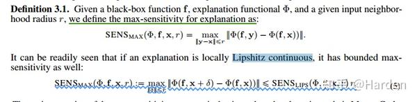
max-sensitivity分数 SENS_{MAX}(\Phi,f,x,r) 的主要好处是可以通过蒙特卡洛采样进行计算。

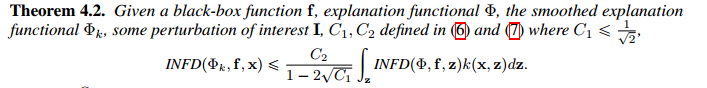
Reducing Sensitivity and Infidelity by Smoothing Explanations

文章指出通过smooth explanation即平滑可解释性函数 \Phi ,可以同时降低sensitivity与infidelity分数。

1.证明降低sensitivity分数

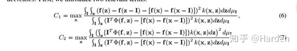
2. 证明降低infidelity分数

Experiment Results

在MNIST, CIFAR-10和ImageNet上的评测对比多种可解释性方法，给出infidelity与sensitivity结果的对比

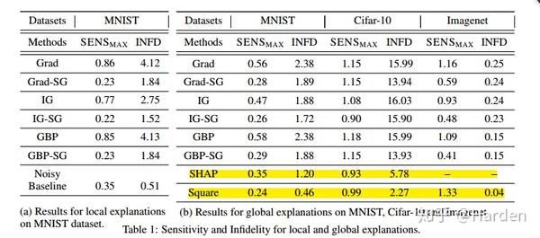
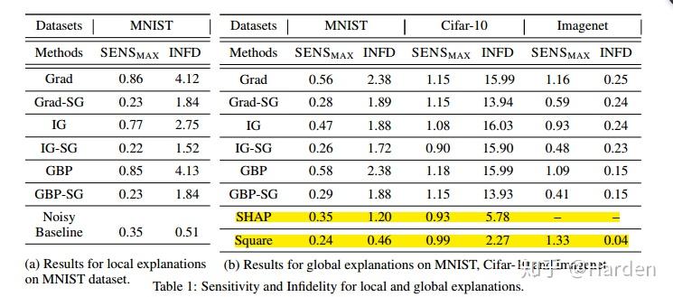
Grad, IG, GBP, SHAP分别是vanilla gradient , integrated gradient, Guided Back-Propagation ^[9] and KernelSHAP ^[10] 等可解释性方法的表示。Grad-SG表示让Grad explanation进行平滑，IG-SG表示让IG explanation进行平滑，GBP-SG表示使GBP explanation进行平滑，Noisy baseline和Square是作者提出的两种新的扰动形式。

从上表可以看出：通过Smooth操作，GBP IG 与Grad等可解释性方法的性能得到了提升，

Noisy baseline和Square两种文章提出的扰动方法，对应的可解释性方法的性能达到最佳。

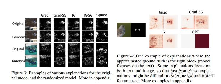
下面是可视化的一些结果展示

参考

1. ^ Ancona, M., Ceolini, E., Öztireli, C., and Gross, M. A unified view of gradient-based attribution methods for deep neural networks. International Conference on Learning Representations,2018.
2. ^ Sundararajan, M., Taly, A., and Yan, Q. Axiomatic attribution for deep networks. In International Conference on Machine Learning, 2017.
3. ^ Daniel Smilkov, Nikhil Thorat, Been Kim, Fernanda B. Viegas, and Martin Wattenberg. 2017. SmoothGrad: ´ removing noise by adding noise. In ICML Workshop on Visualization for Deep Learning.
4. ^ Shrikumar, A., Greenside, P., and Kundaje, A. Learning important features through propagating activation differences. International Conference on Machine Learning, 2017.
5. ^ Bach, S., Binder, A., Montavon, G., Klauschen, F., Müller, K.-R., and Samek, W. On pixel-wise explanations for non-linear classifier decisions by layer-wise relevance propagation. PloS one, 10(7):e0130140, 2015.
6. ^ Shrikumar, A., Greenside, P., Shcherbina, A., and Kundaje, A. Not just a black box: Learning important features through propagating activation differences. arXiv preprint arXiv:1605.01713, 2016.
7. ^ Zeiler, M. D. and Fergus, R. Visualizing and understanding convolutional networks. In European conference on computer vision, pp. 818–833. Springer, 2014.
8. ^ Lundberg, S. M. and Lee, S.-I. A unified approach to interpreting model predictions. In Advances in Neural Information Processing Systems, pp. 4765–4774, 2017.
9. ^ vanilla gradient [37], integrated gradient [43], Guided Back-Propagation [41], and KernelSHAP [25]
10. ^ Lundberg, S. M. and Lee, S.-I. A unified approach to interpreting model predictions. In Advances in Neural Information Processing Systems, pp. 4765–4774, 2017.