|
|
|


用matlab画有限长均匀带电线段的电场线,电势分布?
关注者
4
被浏览
9,371
登录后你可以
不限量看优质回答
私信答主深度交流
精彩内容一键收藏


静电场方程
有限长均匀带电线段的静电场满足方程:
\nabla \cdot \boldsymbol{E} = \dfrac{\rho}{\varepsilon} , \tag{1-1} 其中 \boldsymbol{E} 是场强矢量; \rho 是电荷密度,在带电体外, \rho = 0 ,在带电体内 \rho 是非零常数; \varepsilon 是介电常数。引入势函数 \varPhi ,使得 \boldsymbol{E} = -\nabla \varPhi ,则
\nabla \cdot \left( -\nabla \varPhi \right) = -\Delta \varPhi = \dfrac{\rho}{\varepsilon} . \tag{1-2} 对于有限长带电线段,使用柱坐标系比较方便。在柱坐标系中,静电场方程为
-\left[ \dfrac{1}{r} \dfrac{\partial}{\partial r} \left( r \dfrac{\partial \Phi}{\partial r} \right) + \dfrac{1}{r^2} \dfrac{\partial^2 \Phi}{\partial \theta^2} + \dfrac{\partial^2 \Phi}{\partial z^2} \right]= \dfrac{\rho}{\varepsilon} . \tag{1-3} 由于 \varPhi 与 \theta 无关,因此方括号中第二项为零。将方括号中第一项展开并化简,得
-\left( \dfrac{\partial^2 \varPhi}{\partial r^2} + \dfrac{\partial^2 \varPhi}{\partial z^2} \right) = \dfrac{1}{r} \dfrac{\partial \varPhi}{\partial r} + \dfrac{\rho}{\varepsilon} . \tag{1-4} 此时问题化为二维情形。
使用 MATLAB 的 PDE Toolbox 求解方程
下面使用 MATLAB 的偏微分方程工具箱 (PDE Toolbox) 求解此方程。当只有一个待求场变量时,PDE Toolbox 可求解的方程为
m \dfrac{\partial^2 u}{\partial t^2} + d \dfrac{\partial u}{\partial t} - \nabla \cdot \left( c \nabla u \right) + a u = f . \tag{2-1} 若 c 是常数,上式在平面问题中的展开形式为
m \dfrac{\partial^2 u}{\partial t^2} + d \dfrac{\partial u}{\partial t} - c \dfrac{\partial^2 u}{\partial x^2} - c \dfrac{\partial^2 u}{\partial y^2} + a u = f . \tag{2-2} 对于我们要求解的柱坐标系中的静电场方程, u = \varPhi , x = z , y = r , m = d = a = 0 , c = 1 , f = \dfrac{1}{r} \dfrac{\partial \varPhi}{\partial r} + \dfrac{\rho}{\varepsilon} 。
创建模型和几何
用来描述几何区域的函数 ComputationField 见文章末尾,函数的写法见
% Uniformly eletrified bar.
% Author: AdamTurner, 2021.06.
% Written in MATLAB R2018a.
% All properties are in SI-units.
clear all;
close all;
clc;
% ---------- Parameters ---------- %
% Geometry Dimensions.
global radiusField radiusBar lengthBar;
radiusField = 1.000;
radiusBar = 0.050;
lengthBar = 0.500;
% Physics.
global epsilon0 electricQ;
epsilon0 = 8.854187817e-12;   % permittivity of vacuum.
electricQ = 1.000;  % electric density.
% ---------- Set PDE Model ---------- %
% Create PDE models.
pdeModel = createpde(1);
% Create geometry.
geometryFromEdges(pdeModel, @ComputationField);
hFigureGeometry = ...
    figure('Name', 'Geometry', 'NumberTitle', 'off');
hAxesGeometry = ...
    axes(hFigureGeometry, 'NextPlot', 'add', ...
         'Box', 'on', ...
         'FontName', 'Times New Roman', 'FontSize', 12);
hGeometry = ...
    pdegplot(pdeModel, 'EdgeLabels', 'on', 'FaceLabels', 'on', 'SubdomainLabels', 'on');
xlabel('$z$', 'Interpreter', 'latex');
ylabel('$r$', 'Interpreter', 'latex');
title('Geometry');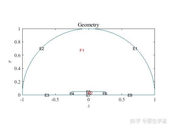

指定边界条件
在第一、二条边界处,我们指定 Dirichlet 边界条件 u = 0 ;在第三、七、八条边界(即对称轴)处,我们指定 Neumann 边界条件 \boldsymbol{n} \cdot \left( \nabla u \right) + q u = g ,其中 q = g = 0 。
% Specify boundary conditions.
applyBoundaryCondition(pdeModel, 'dirichlet', 'Edge', [1, 2], ...
                        'u', 0.000);
applyBoundaryCondition(pdeModel, 'neumann', 'Edge', [3, 7, 8], ...
                       'q', 0.000, 'g', 0.000);
指定方程系数
如前所述, m = d = a = 0 , c = 1 , f = \dfrac{1}{r} \dfrac{\partial \varPhi}{\partial r} + \dfrac{\rho}{\varepsilon} 。由于 f 不是常数,我们提供一个函数描述它(见文章末尾),函数的写法见
% Specify the PDE coefficients.
m = 0.000;
d = 0.000;
c = 1.000;
a = 0.000;
f = @fCoefficient;
specifyCoefficients(pdeModel, ...
                    'm', m, ...
                    'd', d, ...
                    'c', c, ...
                    'a', a, ...
                    'f', f);
创建网格
% Generate mesh.
hMax = 0.250 * min([radiusField, radiusBar, lengthBar]);
generateMesh(pdeModel, 'Hmax', hMax);
hFigureMesh = ...
figure('Name', 'Meshes', 'NumberTitle', 'off');
hAxesMesh = ...
axes(hFigureMesh
, 'NextPlot', 'add', ...
'Box', 'on', ...
'FontName', 'Times New Roman', 'FontSize', 12);
hMesh = ...
pdeplot(pdeModel);
xlabel('$z$', 'Interpreter', 'latex');
ylabel('$r$', 'Interpreter', 'latex');
title('Meshes');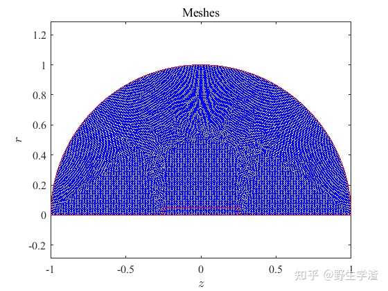

求解
% ---------- Solve ---------- %
pdeResult = solvepde(pdeModel);
绘制结果
对二维问题的数值解进行后处理的方法参见我的一篇文章
% ---------- Plot Result ---------- %
Phi = pdeResult.NodalSolution;
Ex = -pdeResult.XGradients;
Ey = -pdeResult.YGradients;
hFigureResult = ...
    figure('Name', 'Result', 'NumberTitle', 'off');
hAxesResult = ...
    axes(hFigureResult, 'NextPlot', 'add', ...
         'Box', 'on', ...
         'FontName', 'Times New Roman', 'FontSize', 12);
hContour = pdeplot(pdeModel, 'XYData', Phi, ...
                'Contour', 'on', ...
                'ColorBar', 'on', 'ColorMap', 'cool');
hAxesResult.NextPlot = 'add';
% Electric field line.
mGrid = 51;
nGrid = 101;
xq = linspace(-radiusField, radiusField, nGrid).';
yq = linspace(0.000, radiusField, mGrid).';
[xq, yq] = meshgrid(xq, yq);
[Exq, Eyq] = evaluateGradient(pdeResult, xq, yq);
Exq = -reshape(Exq, mGrid, nGrid);
Eyq = -reshape(Eyq, mGrid, nGrid);
xBar = [-0.500, -0.500, 0.500, 0.500] * lengthBar;
yBar = [0.000, 1.000, 1.000, 0.000] * radiusBar;
sBar = [0.000, radiusBar, radiusBar + lengthBar, 2 * radiusBar + lengthBar];
xStart = interp1(sBar, xBar, linspace(0.000, sBar(end), 21), 'linear');
yStart = interp1(sBar, yBar, linspace(0.000, sBar(end), 21), 'linear');
hStream = ...
    streamline(xq, yq, Exq, Eyq, xStart, yStart, 0.010 * radiusField);
nStream = numel(hStream);
for ii = 1 : nStream
    set(hStream(ii), 'LineStyle', '--', 'Color', 'black');
end     % /* for ii */
hBoundary = ...
    plot(hMesh(2).XData, hMesh(2).YData, ...
         'LineWidth', 0.500, 'LineStyle', '-', 'Color', 'red');
xlabel('$z$', 'Interpreter', 'latex');
ylabel('$r$', 'Interpreter', 'latex');
title('$\Phi$', 'Interpreter', 'latex');

将局部放大:
axis([-lengthBar, lengthBar, 0.000, 1.500 * lengthBar]);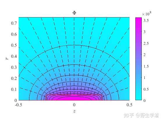

函数
ComputationField.m
% Geometry of computation field.
% Author: AdamTurner, 2021.06.
% Written in MATLAB R2018a.
function varargout = ComputationField(bs, s)
    global radiusField radiusBar lengthBar;
    switch nargin
        case 0
            x = 8;  % number of boundary segments.
            varargout = {x};
            return;
        case 1
            d = [0.000, 0.500 * pi, 1, 0; ...
                 0.500 * pi, pi, 1, 0; ...
                 0.000, 1.000, 1, 0; ...
                 0.000, 1.000, 1, 2; ...
                 0.000, 1.000, 1, 2; ...
                 0.000, 1.000, 1, 2; ...
                 0.000, 1.000, 0, 2; ...
                 0.000, 1.000, 1, 0].';
             x = d(:, bs);
             varargout = {x};
             return;
        case 2
            % starting points.
            x1 = [radiusField, ...
                  0.000, ...
                  -radiusField, ...
                  -0.500 * lengthBar, ...
                  -0.500 * lengthBar, ...
                  0.500 * lengthBar, ...
                  0.500 * lengthBar, ...
                  0.500 * lengthBar].';
            y1 = [0.000, ...
                  radiusField, ...
                  0.000, ...
                  0.000, ...
                  radiusBar, ...
                  radiusBar, ...
                  0.000, ...
                  0.000].';
            % ending points.
            x2 = [0.000, ...
                  -radiusField, ...
                  -0.500 * lengthBar, ...
                  -0.500 * lengthBar, ...
                  0.500 * lengthBar, ...
                  0.500 * lengthBar, ...
                  -0.500 * lengthBar, ...
                  radiusField].';
            y2 = [radiusField, ...
                  0.000, ...
                  0.000, ...
                  radiusBar, ...
                  radiusBar, ...
                  0.000, ...
                  0.000, ...
                  0.000].';
            x = zeros(size(s));
            y = zeros(size(s));
            if numel(bs) == 1
                bs = bs * ones(size(s));
            end     % /* if numel(bs) == 1
            % Edge 1 and 2 (the circular arcs)
            idxCircle = find((bs == 1) | (bs == 2));
            x(idxCircle) = radiusField * cos(s(idxCircle));
            y(idxCircle) = radiusField * sin(s(idxCircle));
            % Edge 3 - 8 (the straight lines)
            idxLine = find((bs ~= 1) & (bs ~= 2));
            for jj = 1 : numel(idxLine)
                x(idxLine(jj)) = x1(bs(idxLine(jj))) + (x2(bs(idxLine(jj))) - x1(bs(idxLine(jj)))) * s(idxLine(jj));
                y(idxLine(jj)) = y1(bs(idxLine(jj))) + (y2(bs(idxLine(jj))) - y1(bs(idxLine(jj)))) * s(idxLine(jj));
            end     % /* for jj */
            varargout = {x, y};
            return;
        otherwise
            error('Too much input arguments!');
    end     % /* switch nargin */
end     % /* ComputationField */
fCoefficient.m
% Specify coefficient f.
% Author: AdamTurner, 2021.06.
% Written in MATLAB R2018a.
function f = fCoefficient(location, state)
    global epsilon0 electricQ;
    nr = length(location.x);    % Number of nodes.
    f = zeros(1, nr);
    idxAxis = abs(location.y) <= eps;