在Python中使用 scipy 执行多维插值方法对比

咖喱乖

算法工程师

1.方法介绍

当已知某些点而不知道具体方程时候，我们通常有两种做法： 拟合或者插值 。

拟合：拟合不要求方程通过所有的已知点，讲究神似，就是整体趋势一致。
插值：插值则是形似，每个已知点都必会穿过，但是高阶会出现龙格库塔现象，所以一般采用分段插值。

scipy 包含各种专用于科学计算中常见问题的工具箱。其不同的子模块对应不同的应用，如插值、积分、优化、图像处理、统计、特殊函数等。 scipy.interpolate为插值模块， 该模块对于从实验数据拟合函数非常有用，可以对不存在测度的点进行评估，该模块基于FITPACK Fortran。

在插值中，二维或者更高维的插值是最值得关注的。目前在scipy.interpolate常用的二维甚至高维插值方法主要有：

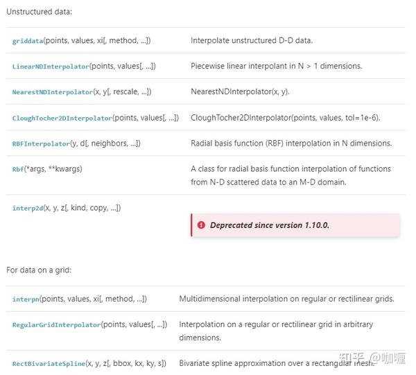
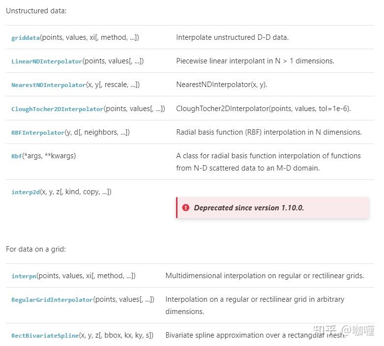
然而，在实际的数据中，由于空间采样的点都是非结构化的实验数据，因此，本文中只介绍一种二维的结构化网格的插值方法，其余都是针对非结构化网格插值方法进行介绍。

RegularGridInterpolator(规则网格化数据插值)
scipy.interpolate.LinearNDInterpolator
scipy.interpolate.NearestNDInterpolator
scipy.interpolate.griddata
scipy.interpolate.RBFInterpolator
scipy.interpolate.Rbf

1.1 RegularGridInterpolator

假设您在 规则网格上有 N 维数据 ，并且您想要对其进行插值。在这种情况下， RegularGridInterpolator 可能会有用。 RegularGridInterpolator 在任意维度的规则或直线网格上进行插值。数据必须在直线网格上定义：即间距均匀或不均匀的 矩形网格 。 支持线性、最近邻、样条插值 。

class scipy.interpolate.RegularGridInterpolator(points, values, method='linear', bounds_error=True, fill_value=nan)

应用案例

from scipy.interpolate import RegularGridInterpolator
def ff(x, y):
    return x**2 + y**2
x, y = np.array([-2, 0, 4]), np.array([-2, 0, 2, 5])
xg, yg = np.meshgrid(x, y, indexing='ij')
data = ff(xg, yg)
interp = RegularGridInterpolator((x, y), data,
                                 bounds_error=False, fill_value=None)
fig = plt.figure()
ax = fig.add_subplot(projection='3d')
ax.scatter(xg.ravel(), yg.ravel(), data.ravel(),
           s=60, c='k', label='data')
xx = np.linspace(-4, 9, 31)
yy = np.linspace(-4, 9, 31)
X, Y = np.meshgrid(xx, yy, indexing='ij')
ax.plot_wireframe(X, Y, interp((X, Y)), rstride=3, cstride=3,
                  alpha=0.4, color='m',label='linear interp')
ax.plot_wireframe(X, Y, ff(X, Y), rstride=3, cstride=3,
                  alpha=0.4,label='ground truth')
plt.legend()
plt.show()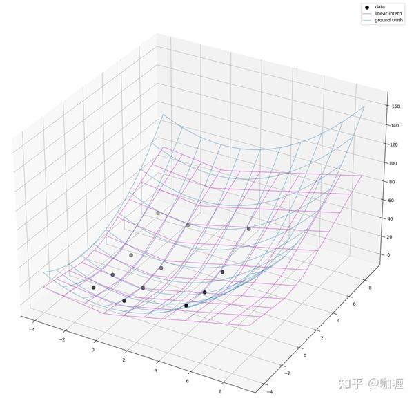

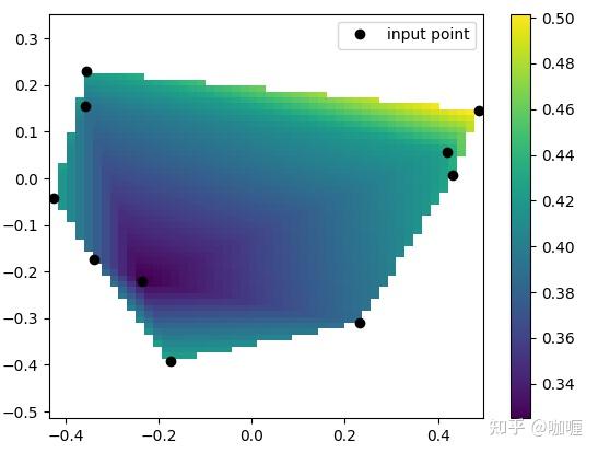
1.2 scipy.interpolate.LinearNDInterpolator

执行N > 1 维中的分段线性插值。

class scipy.interpolate.LinearNDInterpolator(points,values,fill_value=np.nan,rescale=False)

应用案例：

from scipy.interpolate import LinearNDInterpolator
import numpy as np
import matplotlib.pyplot as plt
rng = np.random.default_rng()
x = rng.random(10) - 0.5
y = rng.random(10) - 0.5
z = np.hypot(x, y)
X = np.linspace(min(x), max(x))
Y = np.linspace(min(y), max(y))
X, Y = np.meshgrid(X, Y)  # 2D grid for interpolation
interp = LinearNDInterpolator(list(zip(x, y)), z)
Z = interp(X, Y)
plt.pcolormesh(X, Y, Z, shading='auto')
plt.plot(x, y, "ok", label="input point")
plt.legend()
plt.colorbar()
plt.axis("equal")
plt.show()

1.3 scipy.interpolate.NearestNDInterpolator

执行N > 1 维中的最近邻插值。

class scipy.interpolate.NearestNDInterpolator(x,y,rescale=False,tree_options=None)

应用举例：

from scipy.interpolate import LinearNDInterpolator,NearestNDInterpolator
import numpy as np
import matplotlib.pyplot as plt
rng = np.random.default_rng()
x = rng.random(10) - 0.5
y = rng.random(10) - 0.5
z = np.hypot(x, y)
X = np.linspace(min(x), max(x))
Y = np.linspace(min(y), max(y))
X, Y = np.meshgrid(X, Y)  # 2D grid for interpolation
interp = NearestNDInterpolator(list(zip(x, y)), z)
Z = interp(X, Y)
plt.pcolormesh(X, Y, Z, shading='auto')
plt.plot(x, y, "ok", label="input point")
plt.legend()
plt.colorbar()
plt.axis("equal")
plt.show()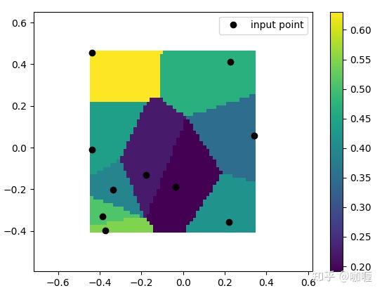

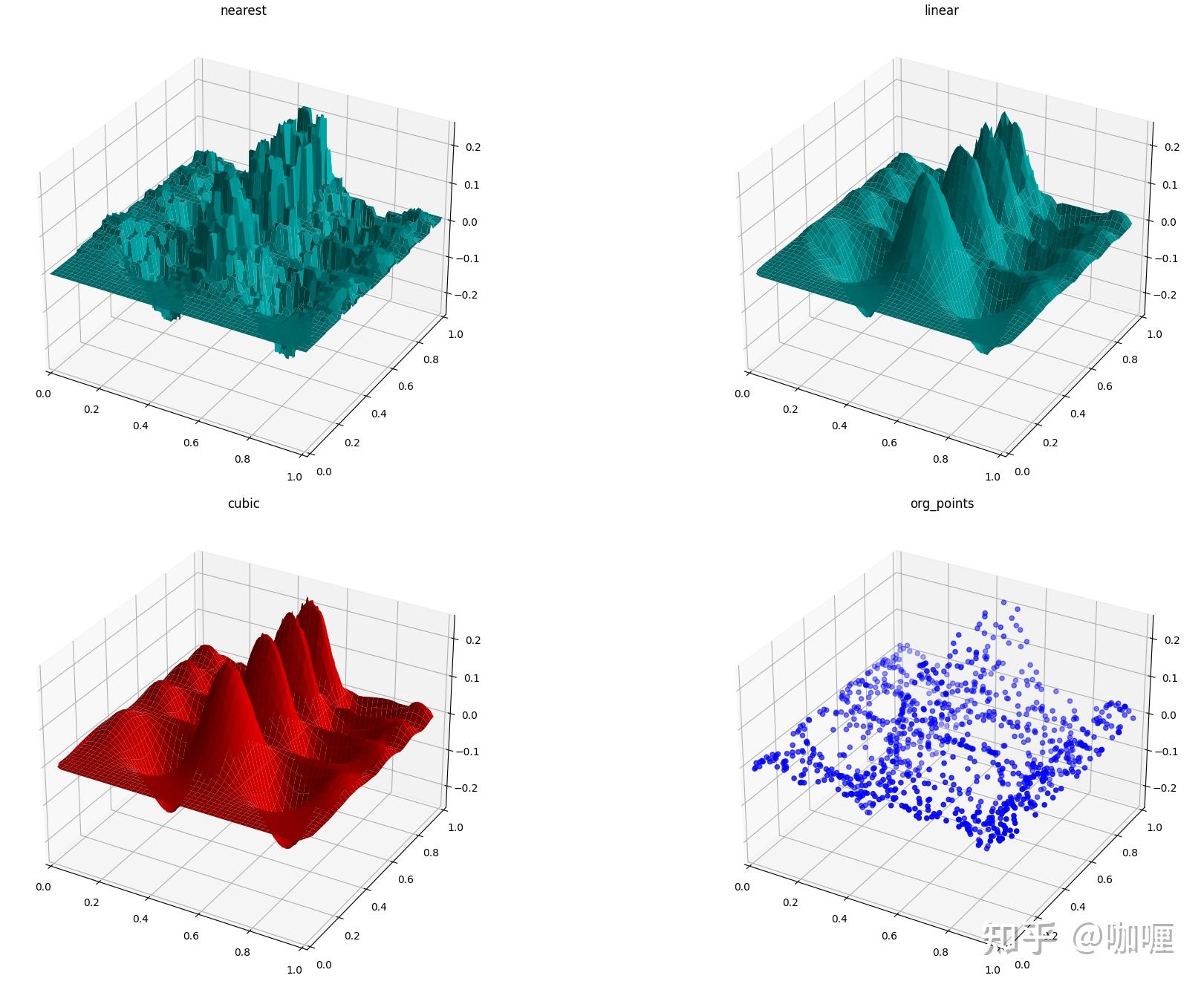
1.4 scipy.interpolate.griddata

假设您有一个基础函数的多维数据 f(x,y) 您只知道不形成规则网格的点的值,假设我们要对二维函数进行插值。 griddata 基于三角剖分，因此适用于非结构化、分散的数据。

scipy.interpolate.griddata(points, values, xi, method='linear', fill_value=nan,rescale=False)

应用案例：

导入依赖库

import matplotlib
import matplotlib.pyplot as plt
from mpl_toolkits.mplot3d.axes3d import Axes3D
import numpy as np
from scipy.interpolate import griddata

生成数据

def func(x, y):
    return x*(1-x)*np.cos(4*np.pi*x) * np.sin(4*np.pi*y**2)**2
grid_x, grid_y = np.mgrid[0:1:100j, 0:1:200j]
points = np.random.rand(1000, 2)
values = func(points[:,0], points[:,1])

插值

grid_z0 = griddata(points, values, (grid_x, grid_y), method='nearest')
grid_z1 = griddata(points, values, (grid_x, grid_y), method='linear')




    

grid_z2 = griddata(points, values, (grid_x, grid_y), method='cubic')

可视化

plt.figure()
ax1 = plt.subplot2grid((2,2), (0,0), projection='3d')
ax1.plot_surface(grid_x, grid_y, grid_z0, color = "c")
ax1.set_xlim3d(0, 1)
ax1.set_ylim3d(0, 1)
ax1.set_zlim3d(-0.25, 0.25)
ax1.set_title('nearest')
ax2 = plt.subplot2grid((2,2), (0,1), projection='3d')
ax2.plot_surface(grid_x, grid_y, grid_z1, color = "c")
ax2.set_xlim3d(0, 1)
ax2.set_ylim3d(0, 1)
ax2.set_zlim3d(-0.25, 0.25)
ax2.set_title('linear')
ax3 = plt.subplot2grid((2,2), (1,0), projection='3d')
ax3.plot_surface(grid_x, grid_y, grid_z2, color = "r")
ax3.set_xlim3d(0, 1)
ax3.set_ylim3d(0, 1)
ax3.set_zlim3d(-0.25, 0.25)
ax3.set_title('cubic')
ax4 = plt.subplot2grid((2,2), (1,1), projection='3d')
ax4.scatter(points[:,0], points[:,1], values,  c= "b")
ax4.set_xlim3d(0, 1)
ax4.set_ylim3d(0, 1)
ax4.set_zlim3d(-0.25, 0.25)
ax4.set_title('org_points')
plt.tight_layout()
plt.show()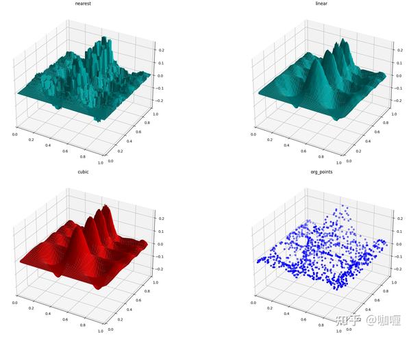

内左上图是method=nearest的插值效果，右上图为method=linear的插值效果，左下图是method=cubic的插值效果，右下图则是已知的多元点集散点图

1.5 scipy.interpolate.RBFInterpolator

执行N 维径向基函数 (RBF) 插值。

class scipy.interpolate.RBFInterpolator(y, d, neighbors=None, smoothing=0.0, kernel='thin_plate_spline', epsilon=None, degree=None)

假设函数可以由RBF(Radial basis functions)径向基函数近似表示，把它代入微分方程并且在某个数据点集上在某种度量下迫使微分方程的误差取最小值，从而决定系数 \alpha_i ，甚至点 x_i ，这个方法在一些实际应用领域也获得了 非常满意的结果，可视化曲线更具光滑。

scipy.interpolate包里有 Rbf函数。径向基函数可用于平滑/插值 N 维的散乱数据，但应谨慎用于观测数据范围外的外推。

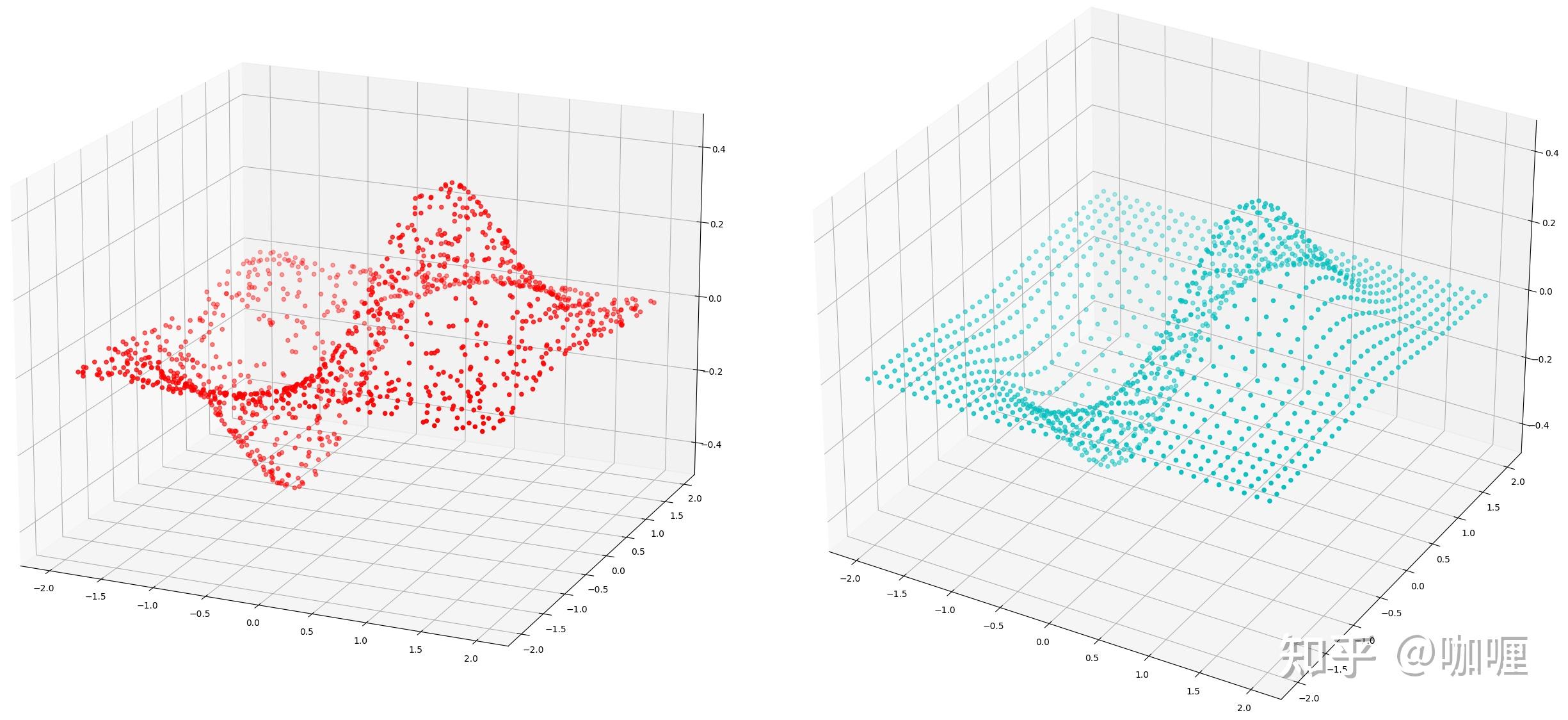
应用举例

import numpy as np
import matplotlib.pyplot as plt
from scipy.interpolate import Rbf, splprep
from matplotlib import cm   
from mpl_toolkits.mplot3d.axes3d import Axes3D
x = np.random.rand(1200) * 4.0 - 2.0
y = np.random.rand(1200) * 4.0- 2.0
z = x * np.exp(-x ** 2 - y ** 2)
rf = Rbf(x, y, z,epsilon = 2)
ti = np.linspace(-2.0, 2.0, 34)
xi, yi = np.meshgrid(ti, ti)
zi = rf(xi, yi)
plt.figure()
ax1 = plt.subplot2grid((1,2), (0,0), projection='3d')
ax1.scatter(x, y, z, color = 'r')
ax2 = plt.subplot2grid((1,2), (0,1), projection='3d')
ax2.scatter(xi, yi, zi,color = 'c')
plt.tight_layout()
plt.show()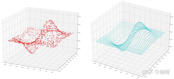

1.6 scipy.interpolate.Rbf

执行用于从 ND 散乱数据到 MD 域的函数的径向基函数插值的类。

class scipy.interpolate.Rbf(*args, **kwargs)

应用举例：

import numpy as np
from scipy.interpolate import Rbf
rng = np.random.default_rng()
x, y, z, d = rng.random((4, 50))
rbfi




    
 = Rbf(x, y, z, d)  # radial basis function interpolator instance
xi = yi = zi = np.linspace(0, 1, 20)
di = rbfi(xi, yi, zi)   # interpolated values
di.shape
>>>(20,)

2.方法对比

针对非结构网格数据插值，似乎上述五种方法均可以，但是到底不同方法的插值效果又何区别，似乎不是太清晰。因此我们重点比较了两种算法常用的（scipy.interpolate.griddata和scipy.interpolate.RBFInterpolator。通过验证的整个流程用来学习如何选择自己合适的插值算法。

为了更好选择数据以及插值目的，我们降以下设置：

我将使它们接受 两种插值任务 和 两种底层函数（要插值的点） 。具体例子将演示二维插值，但可行的方法适用于任意维度。每种方法都提供了多种插值；在所有情况下，我都会使用三次插值。重要的是要注意，无论何时使用插值，与原始数据相比都会引入偏差，并且所使用的特定方法会影响最终得到的伪像。

这 两个插值任务 将是：

上采样 （输入数据在矩形网格上，输出数据在更密集的网格上）
将 分散数据插值 到规则网格上

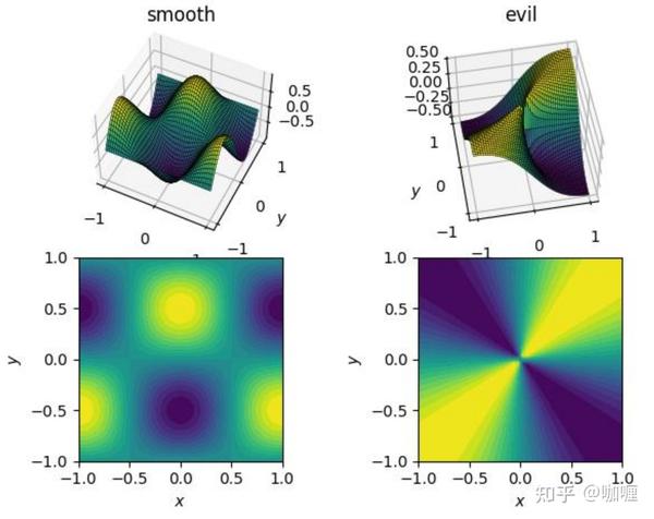
这 两个底层函数 将是：

连续光滑的函数： cos(pi*x)*sin(pi*y)
非连续光滑函数: x*y / (x^2 + y^2)

2.1 光滑函数上采样插值测试

import numpy as np
import scipy.interpolate as interp
# auxiliary function for mesh generation
def gimme_mesh(n):
    minval = -1
    maxval =  1
    # produce an asymmetric shape in order to catch issues with transpositions
    return np.meshgrid(np.linspace(minval, maxval, n),
                       np.linspace(minval, maxval, n + 1))
# set up underlying test functions, vectorized
def fun_smooth(x, y):
    return np.cos(np.pi*x) * np.sin(np.pi*y)
def fun_evil(x, y):
    # watch out for singular origin; function has no unique limit there
    return np.where(x**2 + y**2 > 1e-10, x*y/(x**2+y**2), 0.5)
# sparse input mesh, 6x7 in shape
N_sparse = 6
x_sparse, y_sparse = gimme_mesh(N_sparse)
z_sparse_smooth = fun_smooth(x_sparse, y_sparse)
# scattered input points, 10^2 altogether (shape (100,))
N_scattered = 10
rng = np.random.default_rng()
x_scattered, y_scattered = rng.random((2, N_scattered**2))*2 - 1
z_scattered_smooth = fun_smooth(x_scattered, y_scattered)
# dense output mesh, 20x21 in shape
N_dense = 20
x_dense, y_dense = gimme_mesh(N_dense)
#griddata
sparse_points = np.stack([x_sparse.ravel(), y_sparse.ravel()], -1)  # shape (N, 2) in 2d
z_dense_smooth_griddata = interp.griddata(sparse_points, z_sparse_smooth.ravel(),
                                          (x_dense, y_dense), method='cubic')  # default method is linear
sparse_points = np.stack([x_sparse.ravel(), y_sparse.ravel()], -1)  # shape (N, 2) in 2d
dense_points = np.stack([x_dense.ravel(), y_dense.ravel()], -1)  # shape (N, 2) in 2d
#RBFInterpolator
zfun_smooth_rbf = interp.RBFInterpolator(sparse_points, z_sparse_smooth.ravel(),
                                         smoothing=0, kernel='cubic')  # explicit default smoothing=0 for interpolation
z_dense_smooth_rbf = zfun_smooth_rbf(dense_points).reshape(x_dense.shape)  # not really a function, but a callable class instance
#visual
grid_x = x_dense
grid_y = y_dense
grid_z0 = z_dense_smooth_griddata
triang = tri.Triangulation(grid_x.ravel(), grid_y.ravel())
plt.figure()
ax1 = plt.subplot2grid((2,2), (0,0), projection='3d')
ax1.plot_surface(grid_x, grid_y, grid_z0,color='c')
ax1.scatter(x_sparse, y_sparse, z_sparse_smooth,  c= "r")
ax1.set_title('griddata')
ax2 = plt.subplot2grid((2,2), (0,1))
ax2.set_aspect('equal')
tcf = ax2.tricontourf(triang, grid_z0.ravel(),color='c')
ax2.ticklabel_format(useOffset=False)
ax2.set_title('griddata')
grid_x = x_dense
grid_y = y_dense
grid_z0 = z_dense_smooth_rbf
ax3 = plt.subplot2grid((2,2), (1,0), projection='3d')
ax3.plot_surface(grid_x, grid_y, grid_z0,color='c')
ax3.scatter(x_sparse, y_sparse, z_sparse_smooth,  c= "r")
ax3.set_title('RBFInterpolator')
ax4 = plt.subplot2grid((2,2), (1,1))
ax4.set_aspect




    
('equal')
tcf = ax4.tricontourf(triang, grid_z0.ravel(),color='c')
ax4.ticklabel_format(useOffset=False)
ax4.set_title('RBFInterpolator')
plt.show()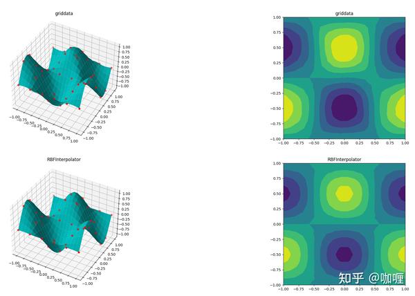

从等值线结果中，差别不是明显！

2.2 非光滑函数上采样插值测试

import numpy as np
import scipy.interpolate as interp
# auxiliary function for mesh generation
def gimme_mesh(n):
    minval = -1
    maxval =  1
    # produce an asymmetric shape in order to catch issues with transpositions
    return np.meshgrid(np.linspace(minval, maxval, n),
                       np.linspace(minval, maxval, n + 1))
# set up underlying test functions, vectorized
def fun_smooth(x, y):
    return np.cos(np.pi*x) * np.sin(np.pi*y)
# sparse input mesh, 6x7 in shape
N_sparse = 6
x_sparse, y_sparse = gimme_mesh(N_sparse)
z_sparse_smooth = fun_smooth(x_sparse, y_sparse)
z_sparse_evil = fun_evil(x_sparse, y_sparse)
# scattered input points, 10^2 altogether (shape (100,))
N_scattered = 10
rng = np.random.default_rng()
x_scattered, y_scattered = rng.random((2, N_scattered**2))*2 - 1
z_scattered_smooth = fun_smooth(x_scattered, y_scattered)
z_scattered_evil = fun_evil(x_scattered, y_scattered)
# dense output mesh, 20x21 in shape
N_dense = 20
x_dense, y_dense = gimme_mesh(N_dense)
#griddata
sparse_points = np.stack([x_sparse.ravel(), y_sparse.ravel()], -1)  # shape (N, 2) in 2d
z_dense_evil_griddata = interp.griddata(sparse_points, z_sparse_evil.ravel(),
                                          (x_dense, y_dense), method='cubic')  # default method is linear
sparse_points = np.stack([x_sparse.ravel(), y_sparse.ravel()], -1)  # shape (N, 2) in 2d
dense_points = np.stack([x_dense.ravel(), y_dense.ravel()], -1)  # shape (N, 2) in 2d
#RBFInterpolator
zfun_evil_rbf = interp.RBFInterpolator(sparse_points, z_sparse_evil.ravel(),
                                       smoothing=0, kernel='cubic')  # explicit default smoothing=0 for interpolation
z_dense_evil_rbf = zfun_evil_rbf(dense_points).reshape(x_dense.shape) 
#visual
grid_x = x_dense
grid_y = y_dense
grid_z0 = z_dense_evil_griddata
triang = tri.Triangulation(grid_x.ravel(), grid_y.ravel())
plt.figure()
ax1 = plt.subplot2grid((2,2), (0,0), projection='3d')
ax1.plot_surface(grid_x, grid_y, grid_z0,color='c')
ax1.scatter(x_sparse, y_sparse, z_sparse_evil,  c= "r")
ax1.set_title('griddata')
ax2 = plt.subplot2grid((2,2), (0,1))
ax2.set_aspect('equal')
tcf = ax2.tricontourf(triang, grid_z0.ravel(),color='c')
ax2.ticklabel_format(useOffset=False)
ax2.set_title('griddata')
grid_x = x_dense
grid_y = y_dense
grid_z0 = z_dense_evil_rbf
triang = tri.Triangulation(grid_x.ravel(), grid_y.ravel())
ax3 = plt.subplot2grid((2,2), (1,0), projection='3d')
ax3.plot_surface(grid_x, grid_y, grid_z0,color='c')
ax3.scatter(x_sparse, y_sparse, z_sparse_evil,  c= "r")
ax3.set_title('RBFInterpolator')
ax4 = plt.subplot2grid((2,2), (1,1))
ax4.set_aspect('equal')
tcf = ax4.tricontourf(triang, grid_z0.ravel(),color='c')
ax4.ticklabel_format(useOffset=False)
ax4.set_title('RBFInterpolator')
plt.show()

从等值线结果中，差别不是明显！

2.3 光滑函数在分散数据插值测试

import




    
 numpy as np
import scipy.interpolate as interp
# auxiliary function for mesh generation
def gimme_mesh(n):
    minval = -1
    maxval =  1
    # produce an asymmetric shape in order to catch issues with transpositions
    return np.meshgrid(np.linspace(minval, maxval, n),
                       np.linspace(minval, maxval, n + 1))
# set up underlying test functions, vectorized
def fun_smooth(x, y):
    return np.cos(np.pi*x) * np.sin(np.pi*y)
def fun_evil(x, y):
    # watch out for singular origin; function has no unique limit there
    return np.where(x**2 + y**2 > 1e-10, x*y/(x**2+y**2), 0.5)
# sparse input mesh, 6x7 in shape
N_sparse = 6
x_sparse, y_sparse = gimme_mesh(N_sparse)
z_sparse_smooth = fun_smooth(x_sparse, y_sparse)
# scattered input points, 10^2 altogether (shape (100,))
N_scattered = 10
rng = np.random.default_rng()
x_scattered, y_scattered = rng.random((2, N_scattered**2))*2 - 1
z_scattered_smooth = fun_smooth(x_scattered, y_scattered)
# dense output mesh, 20x21 in shape
N_dense = 20
x_dense, y_dense = gimme_mesh(N_dense)
#griddata
sparse_points = np.stack([x_scattered.ravel(), y_scattered.ravel()], -1)  # shape (N, 2) in 2d
z_dense_smooth_griddata = interp.griddata(sparse_points, z_scattered_smooth.ravel(),
                                          (x_dense, y_dense), method='cubic')  # default method is linear
#RBFInterpolator
sparse_points = np.stack([x_scattered.ravel(), y_scattered.ravel()], -1)  # shape (N, 2) in 2d
dense_points = np.stack([x_dense.ravel(), y_dense.ravel()], -1)  # shape (N, 2) in 2d
zfun_smooth_rbf = interp.RBFInterpolator(sparse_points, z_scattered_smooth.ravel(),
                                         smoothing=0, kernel='cubic')  # explicit default smoothing=0 for interpolation
z_dense_smooth_rbf = zfun_smooth_rbf(dense_points).reshape(x_dense.shape)  # not really a function, but a callable class instance
#visual
grid_x = x_dense
grid_y = y_dense
grid_z0 = z_dense_smooth_griddata
triang = tri.Triangulation(grid_x.ravel(), grid_y.ravel())
plt.figure()
ax1 = plt.subplot2grid((2,2), (0,0), projection='3d')
ax1.plot_surface(grid_x, grid_y, grid_z0,color='c')
ax1.scatter(x_scattered, y_scattered, z_scattered_smooth,  c= "r")
ax1.set_title('griddata')
ax2 = plt.subplot2grid((2,2), (0,1))
ax2.set_aspect('equal')
ax2.ticklabel_format(useOffset=False)
ax2.contourf(grid_x,grid_y,grid_z0)
ax2.set_title('griddata')
grid_x = x_dense
grid_y = y_dense
grid_z0 = z_dense_smooth_rbf
ax3 = plt.subplot2grid((2,2), (1,0), projection='3d')
ax3.plot_surface(grid_x, grid_y, grid_z0,color='c')
ax3.scatter(x_scattered, y_scattered, z_scattered_smooth,  c= "r")
ax3.set_title('RBFInterpolator')
ax4 = plt.subplot2grid((2,2), (1,1))
ax4.set_aspect('equal')
ax4.tricontourf(triang, grid_z0.ravel(),color='c')
ax4.ticklabel_format(useOffset=False)
ax4.set_title('RBFInterpolator')
plt.show()

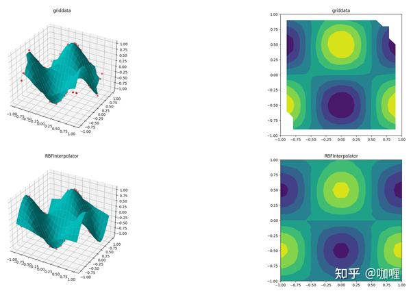
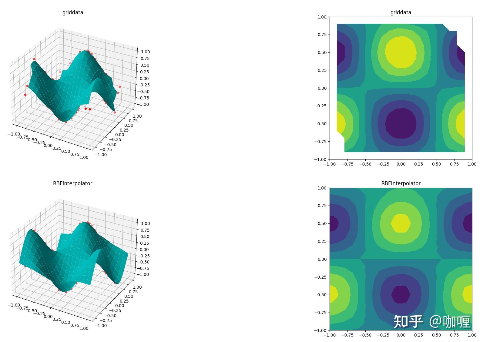
从等值线结果中， RBFInterpolator更优！

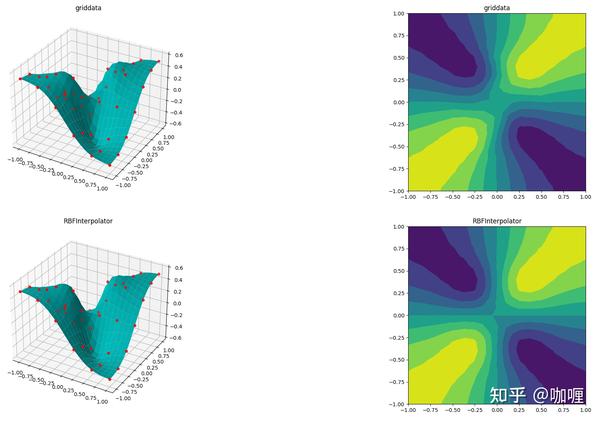
2.4 非光滑函数在分散数据插值测试

import numpy as np
import scipy.interpolate as interp
# auxiliary function for mesh generation
def gimme_mesh(n):
    minval = -1
    maxval =  1
    # produce an asymmetric shape in order to catch issues with transpositions
    return np.meshgrid(np.linspace(minval, maxval, n),
                       np.linspace(minval, maxval, n + 1))
# set up underlying test functions, vectorized
def fun_smooth(x, y):
    return np.cos(np.pi*x) * np.sin(np.pi*y)
def fun_evil(x, y):
    # watch out for singular origin; function has no unique limit there
    return np.where(x**2 + y**2 > 1e-10, x*y/(x**2+y**2), 0.5)
# sparse input mesh, 6x7 in shape
N_sparse = 6
x_sparse, y_sparse = gimme_mesh(N_sparse)
z_sparse_smooth = fun_evil(x_sparse, y_sparse)
# scattered input points, 10^2 altogether (shape (100,))
N_scattered = 10
rng = np.random.default_rng()
x_scattered, y_scattered = rng.random((2, N_scattered**2))*2 - 1
z_scattered_smooth = fun_evil(x_scattered, y_scattered)
# dense output mesh, 20x21 in shape
N_dense = 20
x_dense, y_dense = gimme_mesh(N_dense)
#griddata
sparse_points = np.stack([x_scattered.ravel(), y_scattered.ravel()], -1)  # shape (N, 2) in 2d
z_dense_smooth_griddata = interp.griddata(sparse_points, z_scattered_smooth.ravel(),
                                          (x_dense, y_dense), method='cubic')  # default method is linear
#RBFInterpolator
sparse_points = np.stack([x_scattered.ravel(), y_scattered.ravel()], -1)  # shape (N, 2) in 2d
dense_points = np.stack([x_dense.ravel(), y_dense.ravel()], -1)  # shape (N, 2) in 2d
zfun_smooth_rbf = interp.RBFInterpolator(sparse_points, z_scattered_smooth.ravel(),
                                         smoothing=0, kernel='cubic')  # explicit default smoothing=0 for interpolation
z_dense_smooth_rbf = zfun_smooth_rbf(dense_points).reshape(x_dense.shape)  # not really a function, but a callable class instance
#visual
grid_x = x_dense
grid_y = y_dense
grid_z0 = z_dense_smooth_griddata
triang = tri.Triangulation(grid_x.ravel(), grid_y.ravel())
plt.figure()
ax1 = plt.subplot2grid((2,2), (0,0), projection='3d')
ax1.plot_surface(grid_x, grid_y, grid_z0,color='c')
ax1.scatter(x_scattered, y_scattered, z_scattered_smooth,  c= "r")
ax1.set_title('griddata')
ax2 = plt.subplot2grid((2,2), (0,1))
ax2.set_aspect('equal')
ax2.ticklabel_format(useOffset=False)
ax2.contourf(grid_x,grid_y,grid_z0)
ax2.set_title('griddata')
grid_x = x_dense
grid_y = y_dense
grid_z0 = z_dense_smooth_rbf
ax3 = plt.subplot2grid((2,2), (1,0), projection='3d')
ax3.plot_surface(grid_x, grid_y, grid_z0,color='c')
ax3.scatter(x_scattered, y_scattered, z_scattered_smooth,  c= "r")
ax3.set_title('RBFInterpolator')