ONNX IR 与 Pytorch2ONNX解析

许也

爱丁堡大学高性能计算和数据科学硕士

ONNX (Open Neural Network Exchange) )是一个开源标准格式，用于表示机器学习模型。换句话说，为不同深度学习模型（Pytrorch / Tensorflow）提供的通用开源格式描述。因此，ONNX定义了一系列常用算子, 用于构建机器学习与深度学习模型。

ONNX provides an open source format for AI models, both deep learning and traditional ML. It defines an extensible computation graph model, as well as definitions of built-in operators and standard data types. Currently we focus on the capabilities needed for inferencing (scoring).

ONNX的目标：

The open standard for machine learning interoperability
ONNX is designed to be an open format by providing a common representation of the computation graph。

这也是为什么选择ONNX的意义：定义机器学习交互的标准，提供通用计算图表示。

所以目前其核心优势就是：

P0 支持多种深度学习框架 BuildModels

P0 支持多种硬件设备，并加速推理 DeployModels

P1 支持模型可视化， Netron 等

P1 支持图优化ONNX optimizer

常见的End2End 样例：Pytorch -> ONNX -> TensorRT / CUDA / CPU

ONNX IR Spec

ONNX为不同的型框架提供模型的通用开源格式描述, 包含了以下几个内容：

可扩展的计算图模型定义extensible computation graph model
标准的数据类型的定义
内置的ONNX operators的定义（被分成了一系列primiter operators和function: 使用其他op组成的是一个sub-grah）

#1（可扩展的计算图模型定义）和 #2 （标准的数据类型的定义）组成了ONNX IR #3 （内置的ONNX operators的定义）

项目文件主要结构：

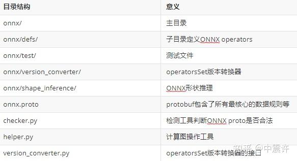
Extensible Computation Graph Model

ONNX提供了可扩展计算图模型，大致构成：ModelProto -> GraphProto -> NodeProto {AttributeProto / ValueInforProto / TensorProto}

通俗理解，ONNX将网络的每一个layer或者每一个op当作节点Node，再由这些Node去构建一个Graph（相当于是一个网络），最后将Graph和这个onnx模型的input信息与output，结合在一起，生成最后一个model，即最终的.onnx的模型。

再反过来说一遍：

ModelProto ，它包含了一些版本信息，生产者信息和一个 GraphProto 。
在 GraphProto 里面又包含了四个 repeated 数组，它们分别是 node ( NodeProto 类型)， input ( ValueInfoProto 类型)， output ( ValueInfoProto 类型)和 initializer ( TensorProto 类型
其中 node 中存放了模型中所有的计算节点， input 存放了模型的输入节点， output 存放了模型中所有的输出节点， initializer 存放了模型的所有权重参数。

Graph Model Example

Model:
graph torch-jit-export (
  %input_xzz[FLOAT, 3000x4]
  %1 = Constant[value = <Scalar Tensor []>]()
  %2 = Gather[axis = 1](%input_xzz, %1)
  %3 = Constant[value = <Scalar Tensor []>]()
  %4 = Gather[axis = 1](%input_xzz, %3)
  %5 = Constant[value = <Scalar Tensor []>]()
  %6 = Gather[axis = 1](%input_xzz, %5)
  %7 = Constant[value = <Scalar Tensor []>]()
  %8 = Gather[axis = 1](%input_xzz, %7)
  %9 = Sub(%6, %2)
  %10 = Constant[value = <Scalar Tensor []>]()
  %11 = Add(%9, %10)
  %12 = Sub(%8, %4)
  %13 = Constant[value = <Scalar Tensor []>]()
  %14 = Add(%12, %13)
  %15 = Constant[value = <Scalar Tensor []>]()
  %16 = Mul(%11, %15)
  %output_xzz = Add(%2, %16)
  %18 = Constant[value = <Scalar Tensor []>]()
  %19 = Mul(%14, %18)
  %20 = Add(%4, %19)
  return %output_xzz, %20, %11, %14
}

Model

是ONNX constuct中最top-level的proto。 protocol buffer 是Google的一种 独立和轻量级 的数据交换格式。以 二进制结构 进行存储。

ONNX使用 protobuf 二进制格式来序列化模型，可以提供更好的传输性能。模型文件model.onnx 是一个protobuf。

protobuf overview

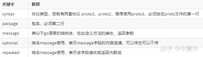
message ModelProto {
  // 每个字段后面数字的，是proto number，理解为每个字段ID
  optional int64 ir_version = 1;
  // 指定模型依赖的operator set集合。
  // OperatorSet定义了可用的operators和their versions.
  // 每一个被模型使用到的operator必须在operator sets中实现
  repeated OperatorSetIdProto opset_import = 8;
  optional string producer_name = 2;
  optional string producer_version = 3;
  optional string domain = 4;
  optional int64 model_version = 5;
  optional string doc_string = 6;   
  // graph proto中存储着用于执行模型的参数化的计算图
  optional GraphProto graph = 7;
};

其中Graph是最为重要的内部proto结构，存储着用于执行模型的参数化的计算图

Graph

Graph定义了模型的计算逻辑：由一系列参数化的Node构成，Node根据他们的inputs和outputs生成了DAG（有向无环图）。

Graph Proto里面有几个重要结构：node / initializer / input / output / value_info

message GraphProto {
  // 图中节点按拓扑顺序排序
  repeated NodeProto node = 1;
  // 图名
  string name = 2;   // namespace Graph
  // 初始化列表，存放计算图的constant input，所以类型是TensorProto
  repeated TensorProto initializer = 5;
  // Initializers (see above) stored in sparse format.
  repeated SparseTensorProto sparse_initializer = 15;
  // A human-readable documentation for this graph. Markdown is allowed.
  string doc_string = 10;
  // 图的 inputs and outputs
  // inputs个数 >=0 
  // ouputs个数 >= 0 
  repeated ValueInfoProto input = 11;
  repeated ValueInfoProto output = 12;
  // Information for the values in the graph. The ValueInfoProto.name's
  // must be distinct. It is optional for a value to appear in value_info list.
  repeated ValueInfoProto value_info = 13;
}

每个Graph必须定义name， types, 以及graph input / graph output信息, 这些信息是静态的。

注意：上述代码最后一行，value_info的信息是onnx shape inference推理出来的，记录了graph中每一个node的shape信息

Node

Example

output: "52"
name: "Constant_50"
op_type: "Constant"
attribute {
  name: "value"
    data_type: 1
    raw_data: "\000\000\200?"
  type: TENSOR
}

计算图构成的多个Node格式化样例：

一个Graph是由Nodes组成的DAG， Node的name / input / output / attribute这四个重要属性定义如下：

message NodeProto {
  repeated string input = 1;    // namespace Value
  repeated string output = 2;   // namespace Value
  // An optional identifier for this node in a graph.
  // op的名字 + id，比如Constant_50
  string name = 3;     // namespace Node
  // 要执行的操作符的符号标识符, op的名字, 例如：Constant
  // The symbolic identifier of the Operator to execute.
  string op_type = 4;  // namespace Operator
  // Additional named attributes.
  repeated AttributeProto attribute = 5;
  ... ...
}

Node input 三种来源：

上一个Node的output，
Graph inputs
Graph initializers

计算图必须使用SSA对于所有的node outputs，意味着要求所有的node output必须唯一，同时要求每一个变量只能准确的被赋值/初始化/定义一次，并且每个变量在使用之前都要定义。如果包含nested subgraph, node output name也必须不同于外部可见的node name

graph inputs / initializers + node output 这些name的出现，属于name的定义definition。例如：每一个Node output将会在计算图中引入一个新的name

graph outpus + nodes input 这些name的出现，属于name的使用use

节点与节点之间是如何定义？

每个计算节点都同样会有input和output这样的两个数组(都是普通的string类型)，通过input和output的指向关系，构建出一个深度学习模型的拓扑图。
最后每个计算节点当中还包含了一个AttributeProto数组，用于描述该节点的属性，例如Conv层的属性包含group，pads和strides等等，具体每个计算节点的属性、输入和输出参考Operators.md文档

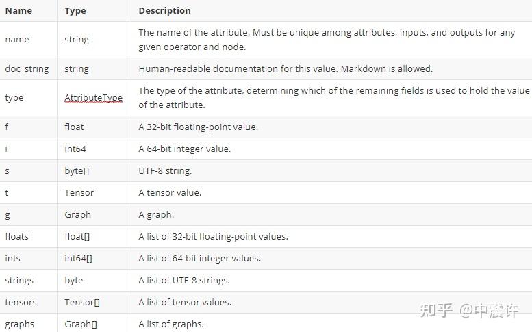
Attribute Values

Attributes value是constant的，因为在模型构建时就被确定了，保存在Node protobuf结构体之中 repeated AttributeProto attribute = 5;

Attribute可以是下述任何一个类型，表明当前node的属性，属性表格如下：

Static Shape

Static Shape只会存在于Graph input / Graph output中，而其他节点的shape信息，需要通过

onnx.shape_inference.infer_shapes(model) 推理出来存放于value_info Proto中

Graph Input / output 样例：

该node的输入为graph input 与 output，所以node信息中具有静态形状信息。可以看到shape形状是3000 * 4

name: "torch-jit-export"
  input {
    name: "input"
    type {
      tensor_type {
        elem_type: 1
        shape {
          dim {
            dim_value: 3000
          dim {
            dim_value: 4
  output {
    name: "output"
    type {
      tensor_type {
        elem_type: 1
        shape {
          dim {
            dim_value: 3000
          dim {
            dim_value: 4
}

然而其他node节点，并没有shape信息

node {
    input: "58"
    input: "59"
    input: "60"
    input: "61"
    output: "output"
    name: "Concat_60"
    op_type: "Concat"
    attribute {
      name: "axis"
      i: 1
      type: INT
    }

inferred Shape

(Inferred Shape) == Input and Ouput Shape of each Node

input and output Shape 是运行时确定，除去Graph input / Graph output，中间node的形状，是需要进行 onnx shape inference才能得到的，存放于Graph value_info Proto中.

经过infer的value info结构, 可以看到上述的input 60，的shape信息，被保存在value info中。

value_info {
    name: "60"
    type {
      tensor_type {
        elem_type: 1
        shape {
          dim {
            dim_value: 3000
          dim {
            dim_value: 1
  }

TensorShape Proto结构：

message TensorShapeProto {
  message Dimension {
    // size of dimension
    oneof value {
      int64 dim_value = 1;
      // string用于表示维度的size并没有限制为特定的数字，对于只关心rank而不关心shape的接口很有用，即动态形状的情况下。
      // shape {dim {dim_param: "my_custom_axis_name"  # axis 0}
      string dim_param = 2;     
      // 当dimension既没有dim_value也没有dim_param，表明当前Node一个未知维度并且和其他未知维度也没关系。
  // 维度：可以是integer 也可以是 symbolic variable(代表未知维度)
  // repeated代表是一个数组：'shape': {'dim': [{'dimValue': '3000'}, {'dimValue': '4'}]}
  repeated Dimension dim = 1;
}

TenshapeProto作为Tenso的子结构

message Tensor {
    int32 elem_type = 1;
    TensorShapeProto shape = 2;
  }

如果shape显示为空的时候，表明为0维的scalar value，这不同于未知维度的张量（动态形状）。如下：constant的outs是一个scalar tensor，并没有shape

node =  {'output': ['4'], 'name': 'Constant_2', 'opType': 'Constant', 'attribute': [{'name': 'value', 't': {'dataType': 7, 'rawData': 'AQAAAAAAAAA='}, 'type': 'TENSOR'}]}
info =  {'name': '4', 'type': {'tensorType': {'elemType': 7, 'shape': {}}}}

Pytorch2ONNX - 定义模型与导出

import torch
import torch.nn as nn
import torch.nn.init as init
import onnx
import onnxruntime
# 1  定义模型
class SuperResolutionNet(nn.Module):
    def __init__(self, upscale_factor, inplace=False):
        super(SuperResolutionNet, self).__init__()
        self.relu = nn.ReLU(inplace=inplace)
        self.conv1 = nn.Conv2d(1, 64, (5, 5), (1, 1), (2, 2))
        self.conv2 = nn.Conv2d(64, 64, (3, 3), (1, 1), (1, 1))
        self.conv3 = nn.Conv2d(64, 32, (3, 3), (1, 1), (1, 1))
        self.conv4 = nn.Conv2d(32, upscale_factor**2, (3, 3), (1, 1), (1, 1))
        self.pixel_shuffle = nn.PixelShuffle(upscale_factor)
        self._initialize_weights()
    def forward(self, x):
        x = self.relu(self.conv1(x))
        x = self.relu(self.conv2(x))
        x = self.relu(self.conv3(x))
        x = self.pixel_shuffle(self.conv4(x))
        return x
    def _initialize_weights(self):
        init.orthogonal_(self.conv1.weight, init.calculate_gain('relu'))
        init.orthogonal_(self.conv2.weight, init.calculate_gain('relu'))
        init.orthogonal_(self.conv3.weight, init.calculate_gain('relu'))
        init.orthogonal_(self.conv4.weight)
# Create the super-resolution model by using the above model definition.
torch_model = SuperResolutionNet(upscale_factor=3)
# set the model to inference mode
# 因为一些算子在不同的表现在inference和training模式下
torch_model.eval()
# Input to the model
x = torch.randn(1, 1, 224, 224, requires_grad=True)
torch_out = torch_model(x)
class Test(nn.Module):
    def __init__(self, upscale_factor, inplace=False):
        super(Test, self).__init__()
        self.test = test
    def forward(




    
self, x):
        x = self.test(x, x)
        return x    
torch_model = SuperResolutionNet(upscale_factor=3)  # Create the model by using the above model definition.
torch_model.eval()                      # set the model to inference mode
# 2  定义input to the model
x = torch.randn(1, 1, 224, 224, requires_grad=True)
torch_out = torch_model(x)
# 3  pytorch导出为onnx格式模型
torch.onnx.export(
    torch_model,  # model being run
    x,  # model input (or a tuple for multiple inputs)
    "super_resolution.onnx",  # where to save the model (can be a file or file-like object)
    verbose=True,
    export_params=True,  # store the trained parameter weights inside the model file
    opset_version=10,  # the ONNX version to export the model to
    do_constant_folding=True,  # whether to execute constant folding for optimization
    input_names=['input'],  # the model's input names
    output_names=['output'],  # the model's output names
    dynamic_axes={
        'input': {
            0: 'batch_size'
        },  # variable length axes
        'output': {
            0: 'batch_size'
    })

torch.onnx.export输出结果:

graph(%input : Float(*, 1, 224, 224, strides=[50176, 50176, 224, 1], requires_grad=1, device=cpu),
      %conv1.weight : Float(64, 1, 5, 5, strides=[25, 25, 5, 1], requires_grad=1, device=cpu),
      %conv1.bias : Float(64, strides=[1], requires_grad=1, device=cpu),
      %conv2.weight : Float(64, 64, 3, 3, strides=[576, 9, 3, 1], requires_grad=1, device=cpu),
      %conv2.bias : Float(64, strides=[1], requires_grad=1, device=cpu),
      %conv3.weight : Float(32, 64, 3, 3, strides=[576, 9, 3, 1], requires_grad=1, device=cpu),
      %conv3.bias : Float(32, strides=[1], requires_grad=1, device=cpu),
      %conv4.weight : Float(9, 32, 3, 3, strides=[288, 9, 3, 1], requires_grad=1, device=cpu),
      %conv4.bias : Float(9, strides=[1], requires_grad=1, device=cpu)):
  %9 : Float(*, 64, 224, 224, strides=[3211264, 50176, 224, 1], requires_grad=1, device=cpu) = onnx::Conv[dilations=[1, 1], group=1, kernel_shape=[5, 5], pads=[2, 2, 2, 2], strides=[1, 1]](%input, %conv1.weight, %conv1.bias) # 
  %10 : Float(*, 64, 224, 224, strides=[3211264, 50176, 224, 1], requires_grad=1, device=cpu) = onnx::Relu(%9) # 
  %11 : Float(*, 64, 224, 224, strides=[3211264, 50176, 224, 1], requires_grad=1, device=cpu) = onnx::Conv[dilations=[1, 1], group=1, kernel_shape=[3, 3], pads=[1, 1, 1, 1], strides=[1, 1]](%10, %conv2.weight, %conv2.bias) # 
  %12 : Float(*, 64, 224, 224, strides=[3211264, 50176, 224, 1], requires_grad=1, device=cpu) = onnx::Relu(%11) # 
  %13 : Float(*, 32, 224, 224, strides=[1605632, 50176, 224, 1], requires_grad=1, device=cpu) = onnx::Conv[dilations=[1, 1], group=1, kernel_shape




    
=[3, 3], pads=[1, 1, 1, 1], strides=[1, 1]](%12, %conv3.weight, %conv3.bias) # 
  %14 : Float(*, 32, 224, 224, strides=[1605632, 50176, 224, 1], requires_grad=1, device=cpu) = onnx::Relu(%13) # 
  %15 : Float(*, 9, 224, 224, strides=[451584, 50176, 224, 1], requires_grad=1, device=cpu) = onnx::Conv[dilations=[1, 1], group=1, kernel_shape=[3, 3], pads=[1, 1, 1, 1], strides=[1, 1]](%14, %conv4.weight, %conv4.bias) # 
  %16 : Long(6, strides=[1], device=cpu) = onnx::Constant[value=  -1    1    3    3  224  224 [ CPULongType{6} ]]()
  %17 : Float(*, 1, 3, 3, 224, 224, device=cpu) = onnx::Reshape(%15, %16)
  %18 : Float(*, 1, 224, 3, 224, 3, device=cpu) = onnx::Transpose[perm=[0, 1, 4, 2, 5, 3]](%17)
  %19 : Long(4, strides=[1], device=cpu) = onnx::Constant[value=  -1    1  672  672 [ CPULongType{4} ]]()
  %output : Float(*, 1, 672, 672, strides=[451584, 451584, 672, 1], requires_grad=1, device=cpu) = onnx::Reshape(%18, %19) # 
  return (%output)

在pytorch.onnx.export这里设置verbose=True，会将整幅计算图进行形状推理，并且打印每个node shape，输出为ONNX格式，

使用ONNX helper工具打印model.graph

model = onnx.load('bbox2offset.onnx')
print('Model:\n\n{}'.format(onnx.helper.printable_graph(model.graph)))
graph torch-jit-export (
  %input[FLOAT, batch_sizex1x224x224]
) initializers (
  %conv1.weight[FLOAT, 64x1x5x5]
  %conv1.bias[FLOAT, 64]
  %conv2.weight[FLOAT, 64x64x3x3]
  %conv2.bias[FLOAT, 64]
  %conv3.weight[FLOAT, 32x64x3x3]
  %conv3.bias[FLOAT, 32]
  %conv4.weight[FLOAT, 9x32x3x3]
  %conv4.bias[FLOAT, 9]
  %9 = Conv[dilations = [1, 1], group = 1, kernel_shape = [5, 5], pads = [2, 2, 2, 2], strides = [1, 1]](%input, %conv1.weight, %conv1.bias)
  %10 = Relu(%9)
  %11 = Conv[dilations = [1, 1], group = 1, kernel_shape = [3, 3], pads = [1, 1, 1, 1], strides = [1, 1]](%10, %conv2.weight, %conv2.bias)
  %12 = Relu(%11)
  %13 = Conv[dilations = [1, 1], group = 1, kernel_shape = [3, 3], pads = [1, 1, 1, 1], strides = [1, 1]](%12, %conv3.weight, %conv3.bias)
  %14 = Relu(%13)
  %15 = Conv[dilations = [1, 1], group = 1, kernel_shape = [3, 3], pads = [1, 1, 1, 1], strides = [1, 1]](%14, %conv4.weight, %conv4.bias)
  %16 = Constant[value = <Tensor>]()
  %17 = Reshape(%15, %16)