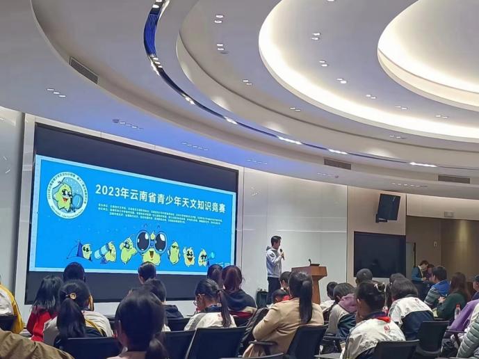
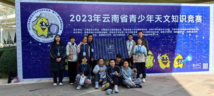
2023年12月15日,由云南省天文学会,云南省天文爱好者协会,云南大学物理与天文学院,云南师范大学物理与电子信息学院等主办的“2023年云南青少年天文知识竞赛”在抚仙湖星空小镇盛大举行;在校领导的支持下,校团委大观天文社派出选手参加了比赛。大观天文社社长马晨作为参赛选手代表在2023年云南青少年天文知识竞赛开始前发言。
在理论与观测两部分的双重考核下,附中学子展现出了超人的竞赛素养与深厚的知识储备,不负众望,共获得个人与团体奖项6个:
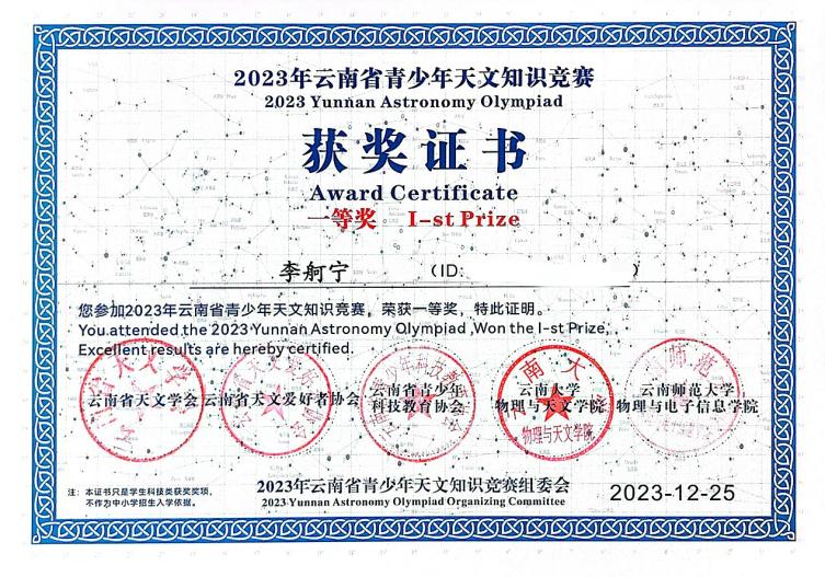
一等奖:高二理1班 李舸宁
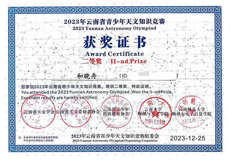
二等奖:高三理8班 和晓舟
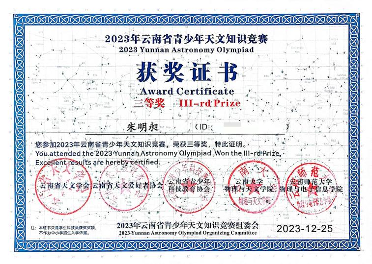
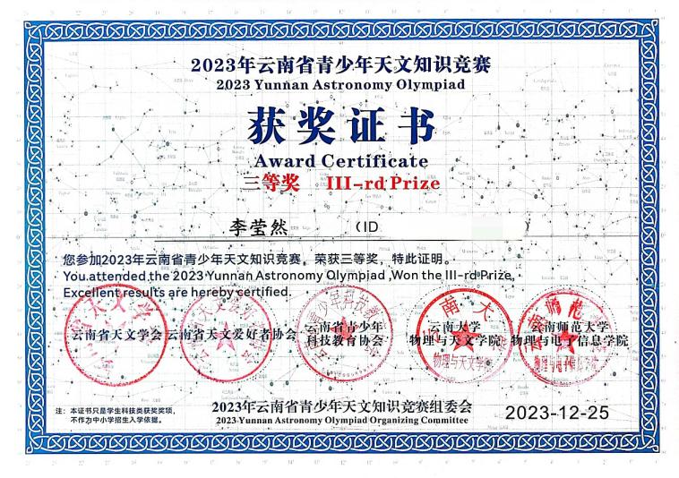
三等奖:高二理2班 朱明昶
高二文5班 李莹然
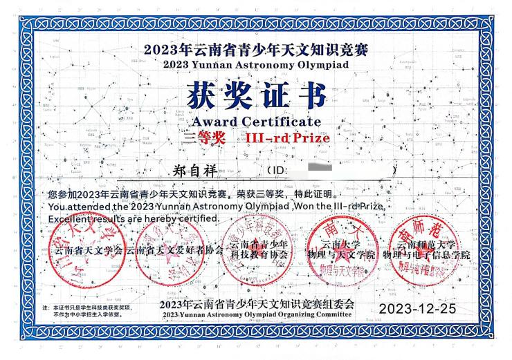
高一2班 郑自祥
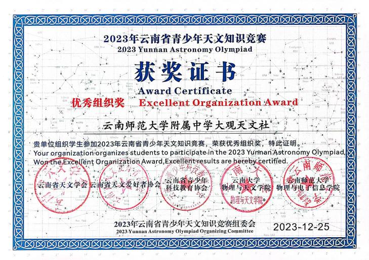
优秀组织奖:云南师范大学附属中学大观天文社
在人类科技不断进步的当下,迈向星空寻求文明进一步的发展是未来的方向。参加天文学竞赛激发兴趣,拓展知识面,利于同学们保持对科学的兴趣和浓厚热情,保持对未知世界强烈的好奇心。在学习和实践中不断弘扬创新精神、锻炼创新思维、提升创新能力,孜孜不倦地追求科学的梦想,坚持不懈地探寻科学的奥秘。
供稿:校团委
撰稿:天文社
一审:赵一青
二审:施加玺
三审:马永文
责编:陈昱嘉
推送:信息中心
学校地址:云南省昆明市五华区洪源路36号(650106)
联系电话:0871-68312226(校办公室)、0871-68313609(教务处)
云南师范大学
云南师大实验中学
云南省招生考试院

