机器学习sklearn之贝叶斯网络实战（一）_tabularcpd_夜风晚凉的博客

贝叶斯网络

贝叶斯网络 、 信念网络 、 贝叶斯模型 或 概率定向无环图形模型 是一种概率图形模型 (一种 统计模型 ), 通过有向无环图 (DAG)表示一组随机变量及其条件依赖关系。
当我们想要表示随机变量之间的因果关系时, 主要使用贝叶斯网络。
贝叶斯网络使用条件概率分布 (CPD) 进行参数化。
网络中的每个节点都使用
建立一个贝叶斯网络模型需要两个参数： 网络模型 及 概率分布
在 pgmpy 中, 定义一个贝叶斯网的流程一般是先建立网络结构, 然后填入相关参数.

from pgmpy.models import BayesianModel
from pgmpy.factors.discrete import TabularCPD
import networkx as nx
from matplotlib import pyplot as plt
%matplotlib inline
# 构建一个网络模型
model = BayesianModel([('D', 'G'),   # 一条有向边，D ---> G
                       ('I', 'G'),   # I ---> G
                       ('G', 'L'),   # G ---> L
                       ('I', 'S')])  # I ---> S
# 设置CPD参数
# variable='D'：节点名为 D，
# variable_card=2：有两种可能的情况，
# values=[[0.6, 0.4]]：概率分别是0.6和0.4
cpd_d = TabularCPD(variable='D', variable_card=2, values=[[0.6, 0.4]])  
# variable='I'：节点名为I
# variable_card=2：有两种可能的情况，
# values=[[0.7, 0.3]]：概率分别是0.7和0.3
cpd_i = TabularCPD(variable='I', variable_card=2, values=[[0.7, 0.3]])
# In pgmpy the colums are the evidences and rows are the states of the variable.
# 在设置G节点时，结构与上图显示的有点不同，这里，列：evidence 行：state，设置参数时，结构如下表：
#    +---------+---------+---------+---------+---------+
#    | diff    | intel_0 | intel_0 | intel_1 | intel_1 |
#    +---------+---------+---------+---------+---------+
#    | intel   | diff_0  | diff_1  | diff_0  | diff_1  |
#    +---------+---------+---------+---------+---------+
#    | grade_0 | 0.3     | 0.05    | 0.9     | 0.5     |
#    +---------+---------+---------+---------+---------+
#    | grade_1 | 0.4     | 0.25    | 0.08    | 0.3     |
#    +---------+---------+---------+---------+---------+
#    | grade_2 | 0.3     | 0.7     | 0.02    | 0.2     |
#    +---------+---------+---------+---------+---------+
# variable='G'：节点名为 G，
# variable_card=3：有两种可能的情况，
# values=[[0.3, 0.05, 0.9,  0.5],
#        [0.4, 0.25, 0.08, 0.3],
#        [0.3, 0.7,  0.02, 0.2]],：针对不同的父节点的情况组合，具有不同的概率分布，如上表
# evidence=['I', 'D']：父节点为 I 和 D，即 I 和 D 指向 G
# evidence_card=[2, 2]：父节点分别有两种可能的情况
cpd_g = TabularCPD(variable='G', variable_card=3, 
                   values=[[0.3, 0.05, 0.9,  0.5],
                           [0.4, 0.25, 0.08, 0.3],
                           [0.3, 0.7,  0.02, 0.2]],
                  evidence=['I', 'D'],
                  evidence_card=[2, 2])
cpd_l = TabularCPD(variable='L', variable_card=2, 
                   values=[[0.1, 0.4, 0.99],
                           [0.9, 0.6, 0.01]],
                   evidence=['G'],
                   evidence_card=[3])
cpd_s = TabularCPD(variable='S', variable_card=2,
                   values=[[0.95, 0.2],
                           [0.05, 0.8]],
                   evidence=['I'],
                   evidence_card=[2])
# Associating the CPDs with the network
# 将概率分布表加入到贝叶斯网络中
model.add_cpds(cpd_d, cpd_i, cpd_g, cpd_l, cpd_s)
# check_model checks for the network structure and CPDs and verifies that the CPDs are correctly 
# defined and sum to 1.
# 验证模型数据的正确性（检测节点是否定义，概率和是否为1）
model.check_model()
# 绘制网络结构图，并附上概率分布表
nx.draw(model,
        with_labels=True,
        node_size=1000,
        font_weight='bold',
        node_color='y',
        pos={"L": [4, 3], "G": [4, 5], "S": [8, 5], "D": [2, 7], "I": [6, 7]})
plt.text(2, 7, model.get_cpds("D"), fontsize=10, color='b')
plt.text(5, 6, model.get_cpds("I"), fontsize=10, color='b')
plt.text(1, 4, model.get_cpds("G"), fontsize=10, color='b')
plt.text(4.2, 2, model.get_cpds("L"), fontsize=10, color='b')
plt.text(7, 3.4




    
, model.get_cpds("S"), fontsize=10, color='b')
plt.title('test')
plt.show()
# We can now call some methods on the BayesianModel object.
# 查看概率分布
model.get_cpds()
[<TabularCPD representing P(D:2) at 0x1df8e84aa58>,
 <TabularCPD representing P(I:2) at 0x1df8e84aa20>,
 <TabularCPD representing P(G:3 | I:2, D:2) at 0x1df92055588>,
 <TabularCPD representing P(L:2 | G:3) at 0x1df8e84aac8>,
 <TabularCPD representing P(S:2 | I:2) at 0x1df8e8d3908>]
# 显示某个节点的概率分布
print(model.get_cpds('G'))
+-----+-----+------+------+-----+
| I   | I_0 | I_0  | I_1  | I_1 |
+-----+-----+------+------+-----+
| D   | D_0 | D_1  | D_0  | D_1 |
+-----+-----+------+------+-----+
| G_0 | 0.3 | 0.05 | 0.9  | 0.5 |
+-----+-----+------+------+-----+
| G_1 | 0.4 | 0.25 | 0.08 | 0.3 |
+-----+-----+------+------+-----+
| G_2 | 0.3 | 0.7  | 0.02 | 0.2 |
+-----+-----+------+------+-----+
model.get_cardinality('G')  # G节点可能的情况有几种（基数）
独立性分析
 
从图中可以看出： 
Causal：在给定B的情况下，A,C被阻断，是独立的$ (A \perp C | B) $
Evidential：在给定B的情况下，A,C是独立的$ (A \perp C | B) $
Common Evidence：在B未知的情况下，A,C是独立的$ (A \perp C | B) $
Common Cause：在给定B的情况下，A,C是独立的$ (A \perp C | B) $ 
import networkx as nx
from matplotlib import pyplot as plt
%matplotlib inline
model2 = BayesianModel([('A', 'B'), ('C', 'B'), ('B', 'D')])
cpd_a = TabularCPD(variable="A", variable_card=2, values=[[0.6, 0.4]])
cpd_c = TabularCPD(variable='C', variable_card=2, values=[[0.7, 0.3]])
cpd_b = TabularCPD(variable='B', variable_card=3, 
                   values=[[0.3, 0.05, 0.9,  0.5],
                           [0.4, 0.25, 0.08, 0.3],
                           [0.3, 0.7,  0.02, 0.2]],
                  evidence=['A', 'C'],
                  evidence_card=[2, 2])
cpd_d = TabularCPD(variable='D', variable_card=2, 
                   values=[[0.1, 0.4, 0.99],
                           [0.9, 0.6, 0.01]],
                   evidence=['B'],
                   evidence_card=[3])
model2.add_cpds(cpd_a, cpd_b, cpd_c, cpd_d)
# 绘制网络结构图
nx.draw(model2,
        with_labels=True,
        node_size=1000,
        font_weight='bold',
        node_color='y',
        pos={"A": [4.9, 4.7], "C": [5.1, 4.7], "B": [5, 4.5], "D": [5, 4.3]})
plt.show()
print("检测模型的正确性：", model2.check_model())
检测模型的正确性： True
print("独立性分析：\n", model2.local_independencies(['D']))
print(model2.local_independencies('B'))  # 没有输出，B与其他节点都相关
print(model2.local_independencies('A'))
print(model2.local_independencies('C'))
独立性分析：
 (D _|_ C, A | B)
(A _|_ C)
(C _|_ A)
第一个案例里的贝叶斯网络的独立性分析
 
model.local_independencies('G')
(G _|_ S | D, I)
model.local_independencies(['D', 'I', 'S', 'G', 'L'])
(D _|_ I, S)
(I _|_ D)
(S _|_ L, D, G | I)
(G _|_ S | D, I)
(L _|_ D, I, S | G)
# Active trail: For any two variables A and B in a network if any change in A influences the values of B then we say
#               that there is an active trail between A and B.
# In pgmpy active_trail_nodes gives a set of nodes which are affected by any change in the node passed in the argument.
model.active_trail_nodes('D')  # 当 D 节点发生变化时，受影响的节点
{'D': {'D', 'G', 'L'}}
model.active_trail_nodes('D', observed='G')  # 当 D 节点发生变化时且 G 节点已知，受影响的节点
{'D': {'D', 'I', 'S'}}
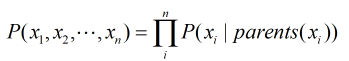
Till now we just have been considering that the Bayesian Network can represent the Joint Distribution without any proof. Now let’s see how to compute the Joint Distribution from the Bayesian Network. 
From the chain rule of probabiliy we know that:联合概率的求解公式如下：
  
Applying the local independence conditions in the above equation we will get:使用上述分子的局部独立条件，得到的联合概率公式为：
  
贝叶斯模型的推断
 
Till now we discussed just about representing Bayesian Networks. Now let’s see how we can do inference in a Bayesian Model and use it to predict values over new data points for machine learning tasks. In this section we will consider that we already have our model. We will talk about constructing the models from data in later parts of this tutorial. 
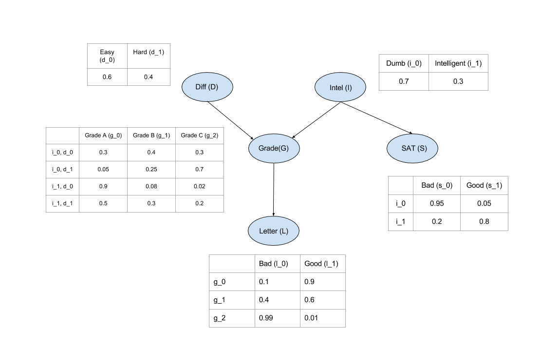
In inference we try to answer probability queries（概率查询） over the network given some other variables. So, we might want to know the probable grade of an intelligent student in a difficult class given that he scored good in SAT. So for computing these values from a Joint Distribution we will have to reduce over the given variables that is  
One of the very basic methods of inference in Graphical Models is Variable Elimination.
 Variable Elimination 
由贝叶斯的联合概率：
  
计算G的概率，我们需要边缘化所有其他变量
  
由局部独立条件化简得：
  
Now since not all the conditional distributions depend on all the variables we can push the summations inside:
 由于并不是所有的条件分布都依赖于所有变量，所以可以变换一下：
  
最后将求和推到里面，可以简化大量的计算
  
from pgmpy.inference import VariableElimination
infer = VariableElimination(model)
print(infer.query(['G'])['G'])
+-----+----------+
| G   |   phi(G) |
+=====+==========+
| G_0 |   0.3620 |
+-----+----------+
| G_1 |   0.2884 |
+-----+----------+
| G_2 |   0.3496 |
+-----+----------+
计算条件分布：  $\sum_L P(L | G) * \sum_S P(S | I=1)$  
在pgmpy 中，只需要传递一个额外的参数evidence。 
print(infer.query(['G'], evidence={'D': 0, 'I': 1})['G'])
+-----+----------+
| G   |   phi(G) |
+=====+==========+
| G_0 |   0.9000 |
+-----+----------+
| G_1 |   0.0800 |
+-----+----------+
| G_2 |   0.0200 |
+-----+----------+
Predicting values from new data points
 
Predicting values from new data points is quite similar to computing the conditional probabilities. We need to query for the variable that we need to predict given all the other features. The only difference is that rather than getting the probabilitiy distribution we are interested in getting the most probable state of the variable. 
当预测新数据时，在给定所有其他特征的基础下，预测的是一个状态值，而不是概率分布 
在pympy中，使用map_query()进行预测 
infer.map_query(['G'])
{'G': 0}
infer.map_query(['G'], evidence={'D': 0, 'I': 1})
{'G': 0}
infer.map_query(['G'], evidence={'D': 0, 'I': 1, 'L': 1, 'S': 1})
{'G': 0}
print(infer.query(['G'], evidence={'D': 0, 'I': 1, 'L': 1, 'S': 1})['G'])
infer.map_query(['G'], evidence={'D': 0, 'I': 1, 'L': 1, 'S': 1})
+-----+----------+
| G   |   phi(G) |
+=====+==========+
| G_0 |   0.9438 |
+-----+----------+
| G_1 |   0.0559 |
+-----+----------+
| G_2 |   0.0002 |
+-----+----------+
{'G': 0}
                                    我只是应用一下说明一下，本文会详细说一下如何通过TabularCPD构造条件概率分布CPD（condition probability distribution）表格，以及各个参数的意义，如果需要完整的贝叶斯网络案例请看这个大神
首先咱是这么个网络
先把点点连起来，前面是箭头出来的事务，后面是箭头到达的事务，如L->N
from pgmpy.models import BayesianNetwork
my_model = BayesianNetwork([('L','N'),('I','N'),('S
                                    从数据中学习贝叶斯网络的CPD参数
正常情况下，我们手头上有的只是数据，对一些CPD的参数值我们通常情况下无法获取，或者获取的代价比较大，那么怎么从数据中学习到贝叶斯网络的参数以及结构呢？这里，我们首先讲解一下参数的学习，即CPD的参数学习。通常采用的方式有：极大似然估计和贝叶斯估计，极大似然估计对样本数量的要求比较高，特别是当数据分布不均匀时，容易发生过拟合线性，为了解决这一问题，通常是采用贝叶...
                                    贝叶斯机器学习Author：louwillMachine Learning Lab  贝叶斯定理是概率模型中最著名的理论之一，在机器学习中也有着广泛的应用。基于贝叶斯理论常用的机器学...
                                    贝叶斯网是一种帮助人们将概率统计应用于复杂领域，进行不确定性推理和数据分析的工具。他起源于人工智能领域的研究。贝叶斯网是一种系统地描述随机变量之间关系的语言。构造贝叶斯网的主要目的是进行概率推理，即计算一些事件发生的概率。贝叶斯网是概率论与图论相结合的产物，它一方面用图论的语言直观的揭示问题结构，另一方面又按照概率论的原则对问题结构加以利用，降低推理的计算复杂度。
贝叶斯网络的构造主要有两种方式：第一种是通过咨询专家手工构造；第二种是通过数据分析获得（讨论利用机器学习的方法...
                                    1、贝叶斯定理P(A∣B)=P(A)P(B∣A)P(B)P(A|B)是已知B发生后A的条件概率，也由于得自B的取值而被称作A的后验概率。P(B|A)是已知A发生后B的条件概率，也由于得自A的取值而被称作B的后验概率。P(A)是A的先验概率或边缘概率。之所以称为”先验”是因为它不考虑任何B方面的因素。P(B)是B的先验概率或边缘概率。贝叶斯定理可表述为：后验概率 = (相似度 * 先验概率) / 标...
                                    首先先复习一下条件概率、全概率、贝叶斯公式的推导过程。并举了三个贝叶斯的相关的例子。贝叶斯网络又称信念网络，是有向无环图模型，是一种概率图形模型。后面会针对贝叶斯网络的实际应用进行说明…
from pgmpy.models import BayesianModel
from pgmpy.factors.discrete.CPD import TabularCPD
import pandas as pd
m = BayesianModel()  # 创建一个贝叶斯网络
m.add_edge('爱情'.
                                    贝叶斯机器学习每一种定理的提出基本都是划时代的，定理的属性代表着它是受逻辑限制的证明为真的陈述，与许多定理一样，可以广泛应用于多种领域，正如热力学中熵的概念，香农则将其迁移到了信息论中，提出了信息论的概念，也有助于后来机器学习决策树中Gini系数的应用。"朴素"的假设了特征x1，x2，…此时，已经得到我们的目标函数，但它还有一个缺陷，P的取值范围在0~1之间，连乘易造成数值下溢的现象，数据看起来会较为不友好，同时因为计算机处理的机制，易将产生数值下溢的数据给记为0，因此我们继续对目标函数进行处理，取log。